Bourdet Derivative Implementation
This document describes the petbox-dca implementation of the Bourdet
three-point derivative smoothing algorithm and its differences from the
original formulation in SPE-12777.
Reference
Bourdet, D., Ayoub, J. A., and Pirard, Y. M. 1989. Use of Pressure Derivative in Well-Test Interpretation. SPE Form Eval 4 (2): 293–302. SPE-12777-PA. https://doi.org/10.2118/12777-PA.
Core Algorithm
The implementation follows Eq. 8 of SPE-12777 exactly. For each data point i, the derivative is computed as the weighted mean of the left and right slopes:
where subscript 1 denotes the left neighbor and subscript 2 denotes the right neighbor, selected as the first points beyond distance L from point i on the log-transformed x-axis.
Implementation Differences
Smoothing parameter units
The original paper defines L in natural-log units (i.e., the
distance on the ln(t) axis). The petbox-dca implementation
defines L in log10 units (decades), consistent with the convention
that production data and well-test plots typically use base-10
logarithmic axes.
To convert between the two conventions:
L_log10 = L_paper / ln(10)
For example, the paper’s L = 0.1 corresponds to L = 0.0434
in this implementation. The typical smoothing range of 0.1–0.5 in
the paper corresponds to approximately 0.04–0.22 in petbox-dca.
Edge handling
SPE-12777 approach. The paper defines three regions:
Left edge (first k1 points): simple forward difference.
Interior (k1 to k2): three-point Bourdet formula.
Right edge (last n - k2 points): simple backward difference.
The transitions between regions can produce discontinuities in the derivative curve. Edge points computed by two-point difference are also more sensitive to noise than interior points.
petbox-dca approach. The three-point formula is applied to all points. When a point lacks a valid neighbor on one side (i.e., it is at the boundary of the data), the formula gracefully degrades:
If only the left neighbor is available (last point): the derivative reduces to the left slope,
Δp₁ / ΔX₁.If only the right neighbor is available (first point): the derivative reduces to the right slope,
Δp₂ / ΔX₂.
This eliminates the edge/interior discontinuity and produces a continuous derivative curve at all points. The one-sided fallback is mathematically equivalent to the paper’s forward/backward difference for points at the data boundaries, but uses the same code path.
Neighbor selection
Both the paper and this implementation select the first data point
beyond distance L. The search is performed using
numpy.searchsorted on the sorted log-transformed x-array, which
provides O(log N) lookup per point and O(N log N) overall, compared
to the O(N²) approach of scanning subarrays for each point.
For L = 0, consecutive points (i - 1 and i + 1) are used
directly, bypassing the search entirely.
Validation
The implementation was validated against the published Table 1 of
SPE-12777 (Buildup 2, 54 data points) at both L = 0 and
L = 0.1 (converted to log10 units).
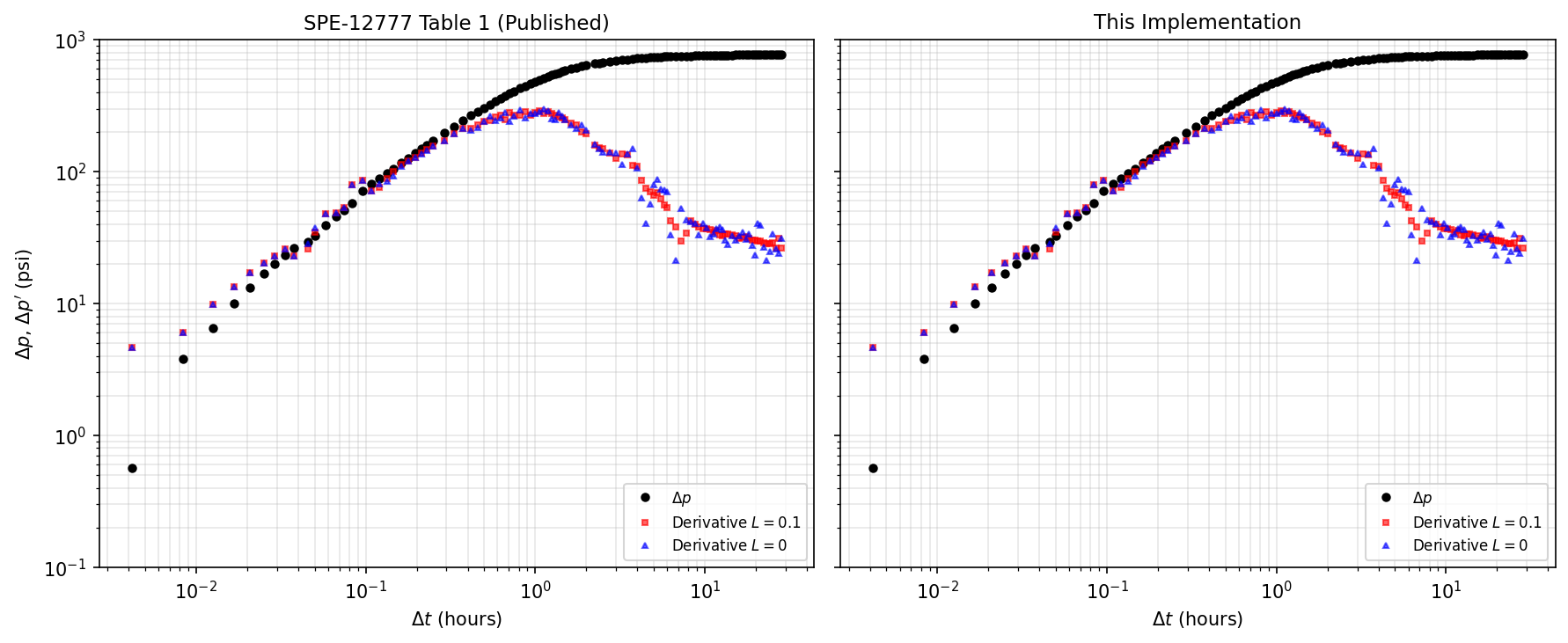
Log-log diagnostic plot comparing published Table 1 derivative
values (left) with petbox-dca output (right). Pressure change
(black circles), unsmoothed derivative (blue triangles, L=0), and
smoothed derivative (red squares, L=0.1).
Interior points (those with full L-windows on both sides) match the published values to within 0.01% relative error. Differences at the data boundaries are expected because the published table is a subset of a larger dataset; the missing points beyond the table boundaries affect the neighbor selection at the edges.
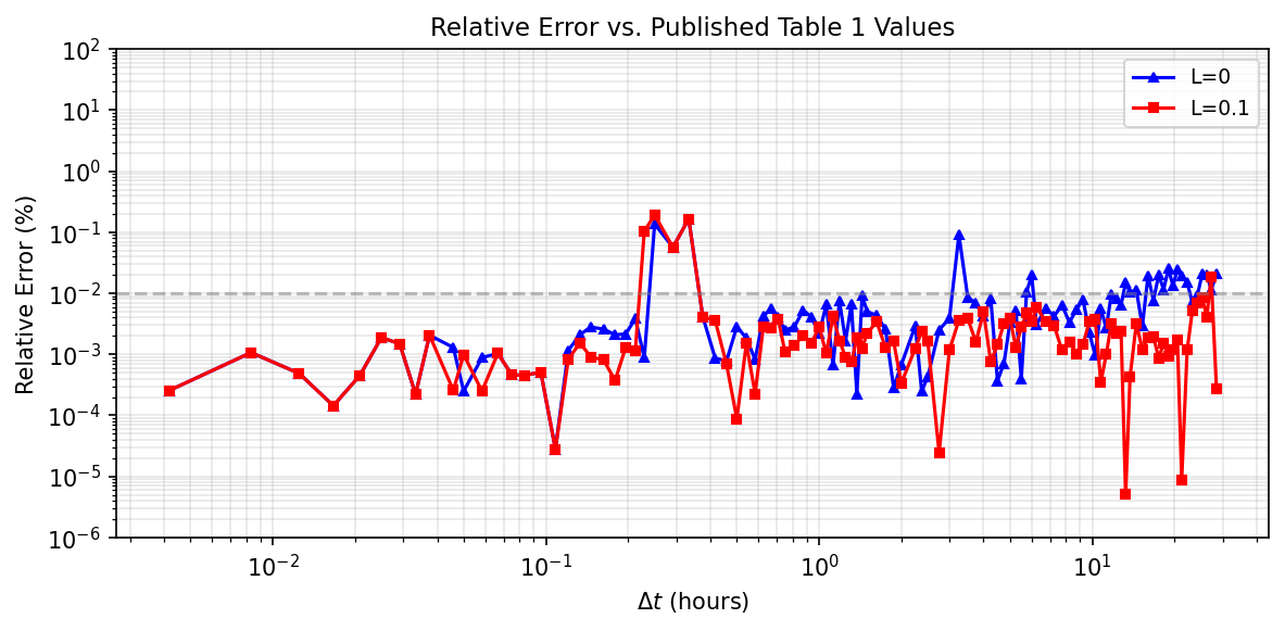
Relative error between the petbox-dca implementation and the
published Table 1 values.
Usage
The smoothing parameter L is specified in log10 cycles:
import numpy as np
from petbox import dca

t = np.array([...])  # time
q = np.array([...])  # rate or pressure

# Unsmoothed derivative: dy / d[ln(x)]
der = dca.bourdet(q, t, L=0.0)

# Smoothed with L = 0.2 log10 cycles
der_smooth = dca.bourdet(q, t, L=0.2)

# Derivative without log-x weighting: dy / dx
der_linear = dca.bourdet(q, t, L=0.2, xlog=False)

# Derivative of log(y): d[ln(y)] / d[ln(x)]
der_loglog = dca.bourdet(q, t, L=0.2, ylog=True)