Detailed Usage Examples

Each model, including the secondary phase models, implements all diagnostic functions. The following is a set of examples to highlight functionality.

from petbox import dca

plt.style.use("seaborn-v0_8-white")
plt.rcParams["font.size"] = 16

# Setup time series for Forecasts and calculate cumulative production of data

# We have this function handy
t = dca.get_time(n=1001)

# Calculate cumulative volume array of data
data_N = np.cumsum(data_q * np.r_[data_t[0], np.diff(data_t)])

# Calculate diagnostic functions D, beta, and b
data_D = -dca.bourdet(data_q, data_t, L=0.35, xlog=False, ylog=True)
data_beta = data_D * data_t
data_b = dca.bourdet(1 / data_D, data_t, L=0.25, xlog=False, ylog=False)

Primary Phase Decline Curve Models

Modified Hyperbolic Model

Robertson, S. 1988. Generalized Hyperbolic Equation. Available from SPE, Richardson, Texas, USA. SPE-18731-MS.

mh = dca.MH(qi=725, Di=0.85, bi=0.6, Dterm=0.2)
q_mh = mh.rate(t)
N_mh = mh.cum(t)
D_mh = mh.D(t)
b_mh = mh.b(t)
beta_mh = mh.beta(t)
N_mh *= data_N[-1] / mh.cum(data_t[-1])

Transient Hyperbolic Model

Fulford, D. S., and Blasingame, T. A. 2013. Evaluation of Time-Rate Performance of Shale Wells using the Transient Hyperbolic Relation. Presented at SPE Unconventional Resources Conference – Canada in Calgary, Alberta, Canda, 5–7 November. SPE-167242-MS. https://doi.org/10.2118/167242-MS.

thm = dca.THM(qi=750, Di=0.8, bi=2, bf=0.5, telf=28)
q_trans = thm.transient_rate(t)
N_trans = thm.transient_cum(t)
D_trans = thm.transient_D(t)
b_trans = thm.transient_b(t)
beta_trans = thm.transient_beta(t)
N_trans *= data_N[-1] / thm.transient_cum(data_t[-1])

Transient Hyperbolic Model Analytic Approximation

Fulford, D.S. 2018. A Model-Based Diagnostic Workflow for Time-Rate Performance of Unconventional Wells. Presented at Unconventional Resources Conference in Houston, Texas, USA, 23–25 July. URTeC-2903036. https://doi.org/10.15530/urtec-2018-2903036.

q_thm = thm.rate(t)
N_thm = thm.cum(t)
D_thm = thm.D(t)
b_thm = thm.b(t)
beta_thm = thm.beta(t)
N_thm *= data_N[-1] / thm.cum(data_t[-1])

Timing Comparison

If performance is a consideration, the approximation is much faster.

>>> %timeit thm.transient_rate(t)
64.9 ms ± 5.81 ms per loop (mean ± std. dev. of 7 runs, 10 loops each)

>>> %timeit thm.rate(t)
86.9 µs ± 5.35 µs per loop (mean ± std. dev. of 7 runs, 10000 loops each)``

Power-Law Exponential Model

Ilk, D., Perego, A. D., Rushing, J. A., and Blasingame, T. A. 2008. Exponential vs. Hyperbolic Decline in Tight Gas Sands – Understanding the Origin and Implications for Reserve Estimates Using Arps Decline Curves. Presented at SPE Annual Technical Conference and Exhibition in Denver, Colorado, USA, 21–24 September. SPE-116731-MS. https://doi.org/10.2118/116731-MS.

Ilk, D., Rushing, J. A., and Blasingame, T. A. 2009. Decline Curve Analysis for HP/HT Gas Wells: Theory and Applications. Presented at SPE Annual Technical Conference and Exhibition in New Orleands, Louisiana, USA, 4–7 October. SPE-125031-MS. https://doi.org/10.2118/125031-MS.

ple = dca.PLE(qi=750, Di=0.1, Dinf=0.00001, n=0.5)
q_ple = ple.rate(t)
N_ple = ple.cum(t)
D_ple = ple.D(t)
b_ple = ple.b(t)
beta_ple = ple.beta(t)
N_ple *= data_N[-1] / ple.cum(data_t[-1])

Stretched Exponential

Valkó, P. P. Assigning Value to Stimulation in the Barnett Shale: A Simultaneous Analysis of 7000 Plus Production Histories and Well Completion Records. 2009. Presented at SPE Hydraulic Fracturing Technology Conference in College Station, Texas, USA, 19–21 January. SPE-119369-MS. https://doi.org/10.2118/119369-MS.

se = dca.SE(qi=715, tau=90.0, n=0.5)
q_se = se.rate(t)
N_se = se.cum(t)
D_se = se.D(t)
b_se = se.b(t)
beta_se = se.beta(t)
N_se *= data_N[-1] / se.cum(data_t[-1])

Duong Model

Duong, A. N. 2001. Rate-Decline Analysis for Fracture-Dominated Shale Reservoirs. SPE Res Eval & Eng 14 (3): 377–387. SPE-137748-PA. https://doi.org/10.2118/137748-PA.

dg = dca.Duong(qi=715, a=2.8, m=1.4)
q_dg = dg.rate(t)
N_dg = dg.cum(t)
D_dg = dg.D(t)
b_dg = dg.b(t)
beta_dg = dg.beta(t)
N_dg *= data_N[-1] / dg.cum(data_t[-1])

Primary Phase Diagnostic Plots

Rate and Cumulative Production Plots

# Rate vs Time
fig = plt.figure(figsize=(15, 7.5))
ax1 = fig.add_subplot(121)
ax2 = fig.add_subplot(122)

ax1.plot(data_t, data_q, "o", mfc="w", label="Data")
ax1.plot(t, q_trans, label="THM Transient")
ax1.plot(t, q_thm, ls="--", label="THM Approx")
ax1.plot(t, q_mh, label="MH")
ax1.plot(t, q_ple, label="PLE")
ax1.plot(t, q_se, label="SE")
ax1.plot(t, q_dg, label="Duong")

ax1.set(xscale="log", yscale="log", ylabel="Rate, BPD", xlabel="Time, Days")
ax1.set(ylim=(1e0, 1e4), xlim=(1e0, 1e4))
ax1.set_aspect(1)
ax1.grid()
ax1.legend()

# Cumulative Volume vs Time
ax2.plot(data_t, data_N, "o", mfc="w", label="Data")
ax2.plot(t, N_trans, label="THM Transient")
ax2.plot(t, N_thm, ls="--", label="THM Approx")
ax2.plot(t, N_mh, label="MH")
ax2.plot(t, N_ple, label="PLE")
ax2.plot(t, N_se, label="SE")
ax2.plot(t, N_dg, label="Duong")

ax2.set(xscale="log", yscale="log", ylim=(1e2, 1e6), xlim=(1e0, 1e4))
ax2.set(ylabel="Cumulative Volume, MBbl", xlabel="Time, Days")
ax2.set_aspect(1)
ax2.grid()
ax2.legend()

plt.savefig(img_path / "model.png")

Diagnostic Function Plots

fig = plt.figure(figsize=(15, 15))
ax1 = fig.add_subplot(221)
ax2 = fig.add_subplot(222)
ax3 = fig.add_subplot(223)
ax4 = fig.add_subplot(224)

# D-parameter vs Time
ax1.plot(data_t, data_D, "o", mfc="w", label="Data")
ax1.plot(t, D_trans, label="THM Transient")
ax1.plot(t, D_thm, ls="--", label="THM Approx")
ax1.plot(t, D_mh, label="MH")
ax1.plot(t, D_ple, label="PLE")
ax1.plot(t, D_se, label="SE")
ax1.plot(t, D_dg, label="Duong")
ax1.set(xscale="log", yscale="log", ylim=(1e-4, 1e0))
ax1.set(ylabel="$D$-parameter, Days$^{-1}$", xlabel="Time, Days")

# beta-parameter vs Time
ax2.plot(data_t, data_D * data_t, "o", mfc="w", label="Data")
ax2.plot(t, beta_trans, label="THM Transient")
ax2.plot(t, beta_thm, ls="--", label="THM Approx")
ax2.plot(t, beta_mh, label="MH")
ax2.plot(t, beta_ple, label="PLE")
ax2.plot(t, beta_se, label="SE")
ax2.plot(t, beta_dg, label="Duong")
ax2.set(xscale="log", yscale="log", ylim=(1e-2, 1e2))
ax2.set(ylabel=r"$\beta$-parameter, Dimensionless", xlabel="Time, Days")

# b-parameter vs Time
ax3.plot(data_t, data_b, "o", mfc="w", label="Data")
ax3.plot(t, b_trans, label="THM Transient")
ax3.plot(t, b_thm, ls="--", label="THM Approx")
ax3.plot(t, b_mh, label="MH")
ax3.plot(t, b_ple, label="PLE")
ax3.plot(t, b_se, label="SE")
ax3.plot(t, b_dg, label="Duong")
ax3.set(xscale="log", yscale="linear", ylim=(0.0, 4.0))
ax3.set(ylabel="$b$-parameter, Dimensionless", xlabel="Time, Days")

# q/N vs Time
ax4.plot(data_t, data_q / data_N, "o", mfc="w", label="Data")
ax4.plot(t, q_trans / N_trans, label="THM Transient")
ax4.plot(t, q_thm / N_thm, ls="--", label="THM Approx")
ax4.plot(t, q_mh / N_mh, label="MH")
ax4.plot(t, q_ple / N_ple, label="PLE")
ax4.plot(t, q_se / N_se, label="SE")
ax4.plot(t, q_dg / N_dg, label="Duong")
ax4.set(xscale="log", yscale="log", ylim=(1e-7, 1e0), xlim=(1e0, 1e7))
ax4.set(ylabel="$q_o / N_p$, Days$^{-1}$", xlabel="Time, Days")

for ax in [ax1, ax2, ax3, ax4]:
    if ax != ax4:
        ax.set(xlim=(1e0, 1e4))
    if ax != ax3:
        ax.set_aspect(1)
    ax.grid()
    ax.legend()


plt.savefig(img_path / "diagnostics.png")

Secondary Phase Decline Curve Models

Power-Law GOR/CGR Model

Fulford, D.S. 2018. A Model-Based Diagnostic Workflow for Time-Rate Performance of Unconventional Wells. Presented at Unconventional Resources Conference in Houston, Texas, USA, 23–25 July. URTeC-2903036. https://doi.org/10.15530/urtec-2018-2903036.

thm = dca.THM(qi=750, Di=0.8, bi=2, bf=0.5, telf=28)
thm.add_secondary(dca.PLYield(c=1.0, m0=-0.1, m=0.8, t0=2 * 365.25 / 12, max=10.0))

Secondary Phase Diagnostic Plots

Rate and Cumluative Production Plots

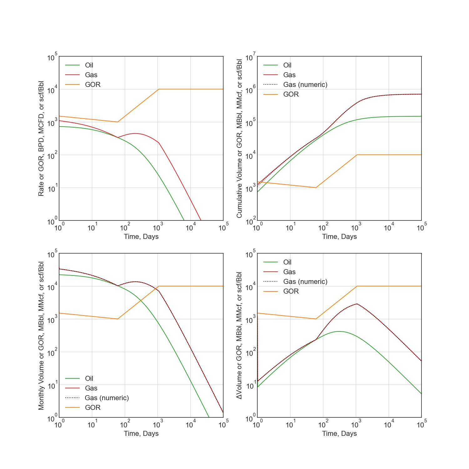
Numeric calculation provided to verify analytic relationships

fig = plt.figure(figsize=(15, 15))
ax1 = fig.add_subplot(221)
ax2 = fig.add_subplot(222)
ax3 = fig.add_subplot(223)
ax4 = fig.add_subplot(224)


# Rate vs Time
q = thm.rate(t)
g = thm.secondary.rate(t)
y = thm.secondary.gor(t)

ax1.plot(t, q, c="C2", label="Oil")
ax1.plot(t, g, c="C3", label="Gas")
ax1.plot(t, y, c="C1", label="GOR")
ax1.set(xscale="log", yscale="log", xlim=(1e0, 1e5), ylim=(1e0, 1e5))
ax1.set(ylabel="Rate or GOR, BPD, MCFD, or Mscf/Bbl", xlabel="Time, Days")


# Cumulative Volume vs Time
q_N = thm.cum(t)
g_N = thm.secondary.cum(t) / 1000.0
_g_N = np.cumsum(g * np.diff(t, prepend=0))

ax2.plot(t, q_N, c="C2", label="Oil")
ax2.plot(t, g_N, c="C3", label="Gas")
ax2.plot(t, _g_N, c="k", ls=":", label="Gas (numeric)")
ax2.plot(t, y, c="C1", label="GOR")
ax2.set(xscale="log", yscale="log", xlim=(1e0, 1e5), ylim=(1e2, 1e7))
ax2.set(ylabel="Rate, Dimensionless", xlabel="Time, Days")
ax2.set(ylabel="Cumulative Volume or GOR, MBbl, MMcf, or Mscf/Bbl", xlabel="Time, Days")


# Time vs Monthly Volume
q_MN = thm.monthly_vol_equiv(t)
g_MN = thm.secondary.monthly_vol_equiv(t) / 1000.0
_g_MN = (
    np.diff(np.cumsum(g * np.diff(t, prepend=0)), prepend=0)
    / np.diff(t, prepend=0)
    * dca.DAYS_PER_MONTH
)

ax3.plot(t, q_MN, c="C2", label="Oil")
ax3.plot(t, g_MN, c="C3", label="Gas")
ax3.plot(t, _g_MN, c="k", ls=":", label="Gas (numeric)")
ax3.plot(t, y, c="C1", label="GOR")
ax3.set(xscale="log", yscale="log", xlim=(1e0, 1e5), ylim=(1e0, 1e5))
ax3.set(ylabel="Monthly Volume or GOR, MBbl, MMcf, or Mscf/Bbl", xlabel="Time, Days")


# Time vs Interval Volume
q_IN = thm.interval_vol(t, t0=0.0)
g_IN = thm.secondary.interval_vol(t, t0=0.0) / 1000.0
_g_IN = np.diff(np.cumsum(g * np.diff(t, prepend=0)), prepend=0)

ax4.plot(t, q_IN, c="C2", label="Oil")
ax4.plot(t, g_IN, c="C3", label="Gas")
ax4.plot(t, _g_IN, c="k", ls=":", label="Gas (numeric)")
ax4.plot(t, y, c="C1", label="GOR")
ax4.set(xscale="log", yscale="log", xlim=(1e0, 1e5), ylim=(1e0, 1e5))
ax4.set(ylabel=r"$\Delta$Volume or GOR, MBbl, MMcf, or Mscf/Bbl", xlabel="Time, Days")

for ax in [ax1, ax2, ax3, ax4]:
    ax.set_aspect(1)
    ax.grid()
    ax.legend()

plt.savefig(img_path / "secondary_model.png")

Diagnostic Function Plots

fig = plt.figure(figsize=(15, 15))
ax1 = fig.add_subplot(221)
ax2 = fig.add_subplot(222)
ax3 = fig.add_subplot(223)
ax4 = fig.add_subplot(224)

# D-parameter vs Time
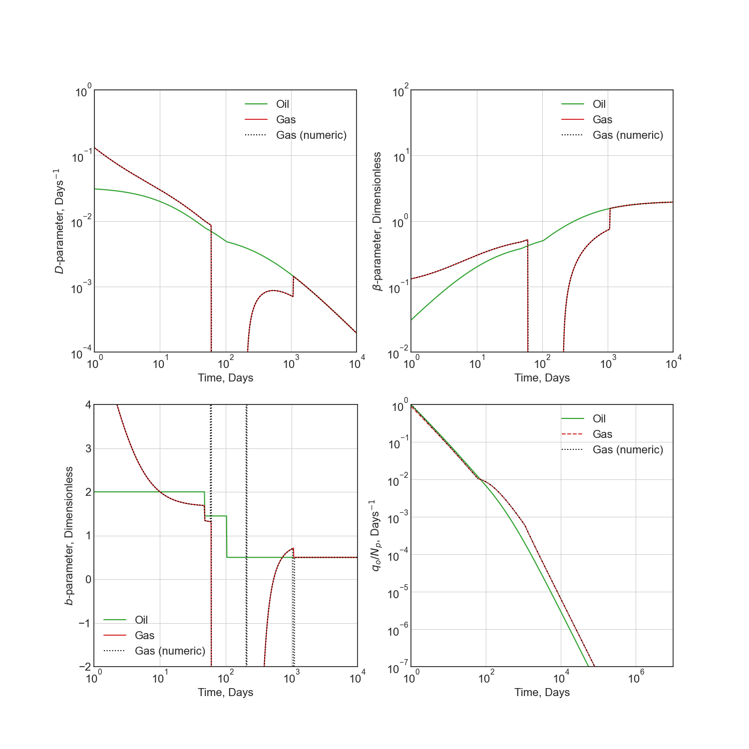
q_D = thm.D(t)
g_D = thm.secondary.D(t)
_g_D = -np.gradient(np.log(thm.secondary.rate(t)), t)

ax1.plot(t, q_D, c="C2", label="Oil")
ax1.plot(t, g_D, c="C3", label="Gas")
ax1.plot(t, _g_D, c="k", ls=":", label="Gas (numeric)")
ax1.set(xscale="log", yscale="log", xlim=(1e0, 1e4), ylim=(1e-4, 1e0))
ax1.set(ylabel="$D$-parameter, Days$^{-1}$", xlabel="Time, Days")

# beta-parameter vs Time
q_beta = thm.beta(t)
g_beta = thm.secondary.beta(t)
_g_beta = _g_D * t

ax2.plot(t, q_beta, c="C2", label="Oil")
ax2.plot(t, g_beta, c="C3", label="Gas")
ax2.plot(t, _g_beta, c="k", ls=":", label="Gas (numeric)")
ax2.set(xscale="log", yscale="log", xlim=(1e0, 1e4), ylim=(1e-2, 1e2))
ax2.set(ylabel=r"$\beta$-parameter, Dimensionless", xlabel="Time, Days")

# b-parameter vs Time
q_b = thm.b(t)
g_b = thm.secondary.b(t)
_g_b = np.gradient(1.0 / _g_D, t)

ax3.plot(t, q_b, c="C2", label="Oil")
ax3.plot(t, g_b, c="C3", label="Gas")
ax3.plot(t, _g_b, c="k", ls=":", label="Gas (numeric)")
ax3.set(xscale="log", yscale="linear", xlim=(1e0, 1e4), ylim=(-2, 4))
ax3.set(ylabel="$b$-parameter, Dimensionless", xlabel="Time, Days")

# q/N vs Time
q_Ng = thm.rate(t) / thm.cum(t)
g_Ng = thm.secondary.rate(t) / thm.secondary.cum(t)
_g_Ng = thm.secondary.rate(t) / np.cumsum(thm.secondary.rate(t) * np.diff(t, prepend=0))

ax4.plot(t, q_Ng, c="C2", label="Oil")
ax4.plot(t, g_Ng, c="C3", ls="--", label="Gas")
ax4.plot(t, _g_Ng, c="k", ls=":", label="Gas (numeric)")
ax4.set(xscale="log", yscale="log", ylim=(1e-7, 1e0), xlim=(1e0, 1e7))
ax4.set(ylabel="$q_o / N_p$, Days$^{-1}$", xlabel="Time, Days")

for ax in [ax1, ax2, ax3, ax4]:
    if ax != ax3:
        ax.set_aspect(1)
    ax.grid()
    ax.legend()

plt.savefig(img_path / "sec_diagnostic_funs.png")

Additional Diagnostic Plots

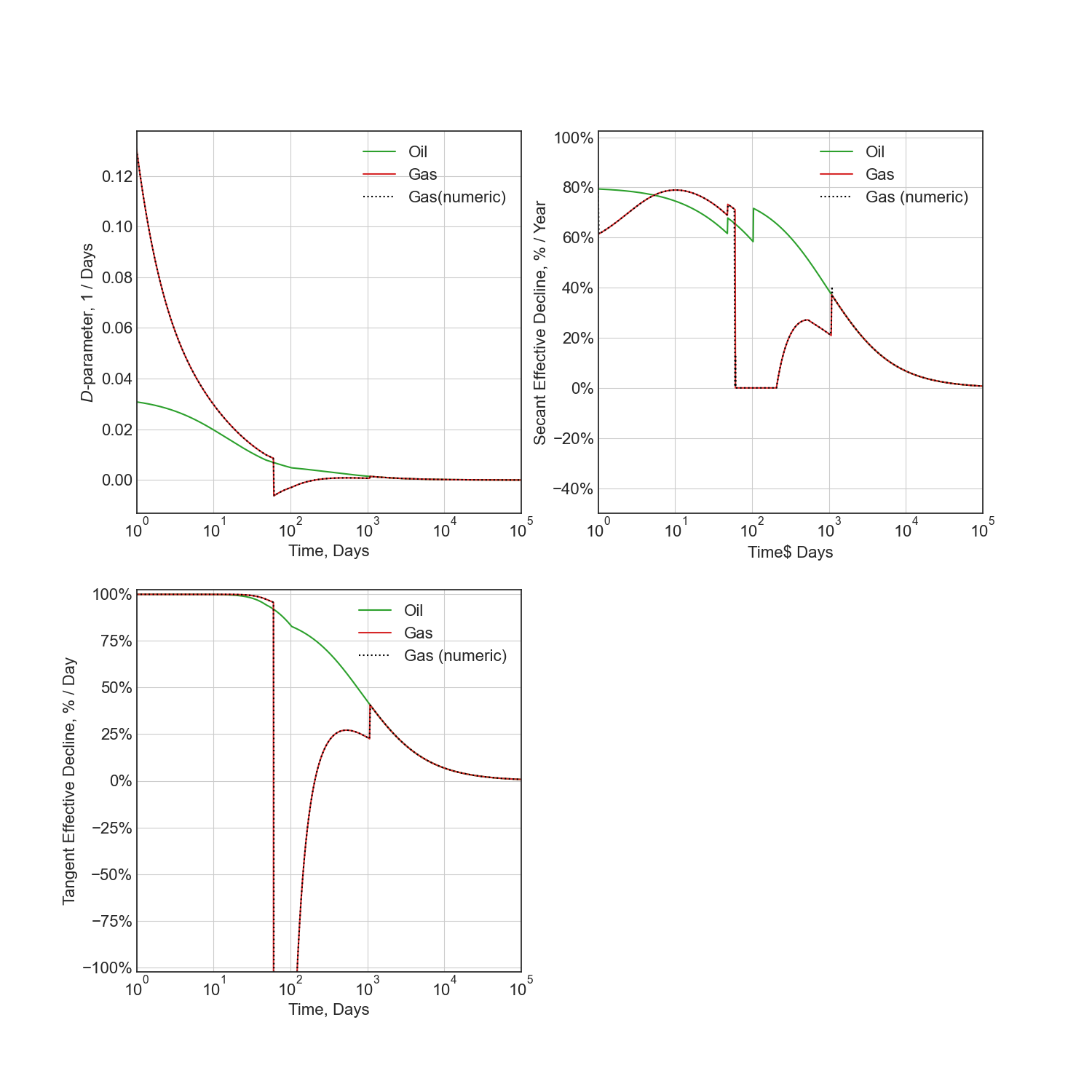
Numeric calculation provided to verify analytic relationships

fig = plt.figure(figsize=(15, 15))
ax1 = fig.add_subplot(221)
ax2 = fig.add_subplot(222)
ax3 = fig.add_subplot(223)

# D-parameter vs Time
q_D = thm.D(t)
g_D = thm.secondary.D(t)
_g_D = -np.gradient(np.log(thm.secondary.rate(t)), t)

ax1.plot(t, q_D, c="C2", label="Oil")
ax1.plot(t, g_D, c="C3", label="Gas")
ax1.plot(t, _g_D, c="k", ls=":", label="Gas(numeric)")
ax1.set(xscale="log", yscale="linear", xlim=(1e0, 1e5), ylim=(None, None))
ax1.set(ylabel="$D$-parameter, 1 / Days", xlabel="Time, Days")

# Secant Effective Decline vs Time
secant_from_nominal = dca.MultisegmentHyperbolic.secant_from_nominal
dpy = dca.DAYS_PER_YEAR

q_Dn = [secant_from_nominal(d * dpy, b) for d, b in zip(q_D, thm.b(t), strict=True)]
g_Dn = [secant_from_nominal(d * dpy, b) for d, b in zip(g_D, thm.secondary.b(t), strict=True)]
_g_Dn = [secant_from_nominal(d * dpy, b) for d, b in zip(_g_D, np.gradient(1 / _g_D, t), strict=True)]

ax2.plot(t, q_Dn, c="C2", label="Oil")
ax2.plot(t, g_Dn, c="C3", label="Gas")
ax2.plot(t, _g_Dn, c="k", ls=":", label="Gas (numeric)")
ax2.set(xscale="log", yscale="linear", xlim=(1e0, 1e5), ylim=(-0.5, 1.025))
ax2.yaxis.set_major_formatter(mpl.ticker.PercentFormatter(xmax=1))
ax2.set(ylabel="Secant Effective Decline, % / Year", xlabel="Time, Days")

# Tangent Effective Decline vs Time
ax3.plot(t, 1 - np.exp(-q_D * dpy), c="C2", label="Oil")
ax3.plot(t, 1 - np.exp(-g_D * dpy), c="C3", label="Gas")
ax3.plot(t, 1 - np.exp(-_g_D * dpy), c="k", ls=":", label="Gas (numeric)")
ax3.set(xscale="log", yscale="linear", xlim=(1e0, 1e5), ylim=(-1.025, 1.025))
ax3.yaxis.set_major_formatter(mpl.ticker.PercentFormatter(xmax=1))
ax3.set(ylabel="Tangent Effective Decline, % / Day", xlabel="Time, Days")

for ax in [ax1, ax2, ax3]:
    ax.grid()
    ax.legend()

plt.savefig(img_path / "sec_decline_diagnostics.png")

Generalized and Inclining Models

A GeneralizedHyperbolic takes an arbitrary number of segments, each continuous in rate and decline with the one before it unless it overrides them. MH is its no-segment case. Segment tuples are length-disambiguated: (t, b), (t, D, b), or (t, q, D, b).

An IncliningHyperbolic requires both Di and bi negative, so the rate rises. It models one period – a build-up – and takes no Dterm, since a rising rate never reaches one. For the physical case, incline to a peak and then decline using both signs of segment.

time_at_rate inverts the rate function, bracketing each segment before inverting it, so it answers both time-to-economic-limit and how far a forecast can be backed up. The pole is simply the infinite-rate limit.

Segment and Rate Inversion Plots

mh_base = dca.MH(qi=725, Di=0.85, bi=0.6, Dterm=0.2)

# Segment tuples are length-disambiguated: (t, b), (t, D, b), or (t, q, D, b). The third
# segment below resets the rate to 120 BPD -- a restimulation -- while inheriting the decline.
gh = dca.GeneralizedHyperbolic.from_segments(
    725,
    0.85,
    1.8,
    [
        (90.0, 1.2),  # exponent only
        (730.0, 0.35, 0.8),  # decline and exponent
        (1825.0, 120.0, None, 0.5),
    ],  # rate reset, decline inherited
    Dterm=0.06,
)

# A flat segment holds the rate; D == 0 requires b == 0.
gh_flat = dca.GeneralizedHyperbolic.from_segments(725, 0.85, 1.8, [(730.0, 0.0, 0.0)])

# `IncliningHyperbolic` requires both Di and bi negative, so the rate rises. It models one
# period -- a build-up -- and takes no Dterm, since a rising rate never reaches one.
ih = dca.IncliningHyperbolic(qi=300, Di=-0.9, bi=-1.0)

# For the physical case, incline to a peak and then decline, using both signs of segment.
peak = dca.GeneralizedHyperbolic.from_segments(300, -0.9, -1.0, [(365.25, 0.75, 1.2)], Dterm=0.08)

# `time_at_rate` inverts the rate function, bracketing each segment before inverting it. The
# pole is simply the infinite-rate limit, so it needs no separate accessor.
econ_limit = 20.0
t_econ = gh.time_at_rate(econ_limit)[0]
t_pole = gh.time_at_rate(np.inf)[0]

fig = plt.figure(figsize=(15, 15))
ax1 = fig.add_subplot(221)
ax2 = fig.add_subplot(222)
ax3 = fig.add_subplot(223)
ax4 = fig.add_subplot(224)

# Rate vs Time -- segmented against the MH baseline
ax1.plot(data_t, data_q, "o", mfc="w", label="Data")
ax1.plot(t, mh_base.rate(t), c="C0", ls="--", label="MH (no segments)")
ax1.plot(t, gh.rate(t), c="C1", label="GeneralizedHyperbolic")
ax1.plot(t, gh_flat.rate(t), c="C4", ls="-.", label="flat segment at 730 d")
ax1.plot(t_econ, econ_limit, "*", c="k", ms=18, label=f"time_at_rate({econ_limit:.0f})")
for t_seg in (90.0, 730.0, 1825.0):
    ax1.axvline(t_seg, c="k", lw=0.5, alpha=0.4)
ax1.set(xscale="log", yscale="log", xlim=(1e0, 1e4), ylim=(1e0, 1e4))
ax1.set(ylabel="Rate, BPD", xlabel="Time, Days")
ax1.set_aspect(1)

# The exponent steps at every segment boundary
ax2.plot(t, mh_base.b(t), c="C0", ls="--", label="MH (no segments)")
ax2.plot(t, gh.b(t), c="C1", label="GeneralizedHyperbolic")
ax2.plot(t, gh_flat.b(t), c="C4", ls="-.", label="flat segment at 730 d")
for t_seg in (90.0, 730.0, 1825.0):
    ax2.axvline(t_seg, c="k", lw=0.5, alpha=0.4)
ax2.set(xscale="log", yscale="linear", xlim=(1e0, 1e4), ylim=(-0.1, 2.1))
ax2.set(ylabel="b Parameter", xlabel="Time, Days")

# Inclining: the pure build-up, and the physical incline-peak-decline
ax3.plot(t, ih.rate(t), c="C2", label="IncliningHyperbolic")
ax3.plot(t, peak.rate(t), c="C3", label="incline, peak, then decline")
ax3.axvline(365.25, c="k", lw=0.5, alpha=0.4)
ax3.set(xscale="log", yscale="log", xlim=(1e0, 1e4), ylim=(1e1, 1e4))
ax3.set(ylabel="Rate, BPD", xlabel="Time, Days")
ax3.set_aspect(1)

# A `GeneralizedPLYield` takes arbitrary breakpoints, and a segment may step the yield
gh_gor = dca.GeneralizedHyperbolic.from_segments(725, 0.85, 1.8, [(90.0, 1.2)])
gh_gor.add_secondary(
    dca.GeneralizedPLYield(
        c=1.2,
        m0=0.0,
        segments=(
            dca.PLYieldSegment(180.0, m=0.6),
            dca.PLYieldSegment(1095.0, c=4.0, m=-0.2),
        ),  # a workover steps the GOR to 4.0
        max=20.0,
    )
)
ax4.plot(t, gh_gor.secondary.gor(t), c="C3", label="GeneralizedPLYield")
for t_seg in (180.0, 1095.0):
    ax4.axvline(t_seg, c="k", lw=0.5, alpha=0.4)
ax4.set(xscale="log", yscale="log", xlim=(1e0, 1e5), ylim=(1e0, 1e1))
ax4.set(ylabel="GOR, Mscf / Bbl", xlabel="Time, Days")

for ax in [ax1, ax2, ax3, ax4]:
    ax.grid()
    ax.legend()

plt.savefig(img_path / "generalized_models.png")