Numerical Integration Method
Several decline curve models in petbox-dca require numerical
integration to compute cumulative volume \(N(t)\) from the rate
function \(q(t)\):
Models with closed-form cumulative solutions (MH, THM, SE, Duong) do not use numerical integration, with one exception: the Stretched Exponential (SE) closed form carries a \(\Gamma(1/n)\) coefficient that overflows for very small \(n\) (\(n \lesssim 0.006\)), where SE falls back to the numerical method described here. The Power-Law Exponential (PLE) model and associated phase models (PLYield) always use this method.
Method
Integration is performed using scipy.integrate.cumulative_trapezoid
on a dense log-spaced grid merged with the requested evaluation times.
Algorithm:
Construct a grid of 10,000 log-spaced points from \(10^{-12}\) to \(t_{max}\), plus a point at \(t = 0\).
Merge the requested \(t\) values into the grid (via
numpy.unique), ensuring exact evaluation at each requested time.Evaluate \(q(t)\) on the full grid in a single vectorized call.
Apply
cumulative_trapezoidto obtain the cumulative integral at every grid point.Extract values at the requested \(t\) indices directly (no interpolation).
Why log-spaced? DCA rate functions typically have their steepest gradients near \(t = 0\) and flatten at late times. A log-spaced grid concentrates evaluation points where the function changes most rapidly, matching the natural scale of the problem. A uniform grid of the same size would under-resolve the early-time region and waste points at late times.
Why merge with t? By including the requested \(t\) values in the integration grid, the cumulative integral is evaluated exactly at those points — no interpolation error is introduced.
Grid Resolution
The default grid uses 10,000 log-spaced points. This was selected by
benchmarking against adaptive quadrature (scipy.integrate.quad with
limit=200) across PLE models spanning mild to steep decline rates:
All cases: \(q_i = 10{,}000\), evaluated at 101 log-spaced points from 1 to 10,000 days. Reference computed with adaptive quadrature (absolute tolerance \(\sim 10^{-14}\)).
The worst-case maximum relative error is 0.00022% (2.2 parts per million), which is well below the uncertainty inherent in empirical decline curve parameters. Mean errors are an order of magnitude smaller.
The grid size is configurable via the n_grid keyword, which flows
through cum(t, n_grid=...) (and the other volume methods). The
log-spaced trapezoid rule converges at second order — each doubling of
n_grid cuts the relative error roughly four-fold — so the knob
trades accuracy for a proportional reduction in grid work. Worst-case
error over the four PLE cases above:
n_grid |
Max Rel Err (%) |
Mean Rel Err (%) |
|---|---|---|
250 |
0.11 |
0.087 |
500 |
0.056 |
0.044 |
1,000 |
0.019 |
0.014 |
2,000 |
0.0054 |
0.0041 |
5,000 |
0.00087 |
0.00068 |
10,000 |
0.00022 |
0.00017 |
20,000 |
0.000056 |
0.000044 |
The default of 10,000 (\(\sim 2 \times 10^{-6}\) relative error) is
unchanged. A smaller value such as 2,000 (\(\sim 5 \times 10^{-5}\))
remains far below the noise in empirical production data, and is a
reasonable choice when integrating repeatedly at moderate accuracy (e.g.
fitting on a fixed t). n_grid must be \(\ge 2\); smaller
values raise ValueError. For typical evaluation arrays the accuracy
is governed by n_grid rather than by the density of the requested
t values — the log-spaced grid dominates the merged integration
grid, so refining t alone does not improve accuracy.
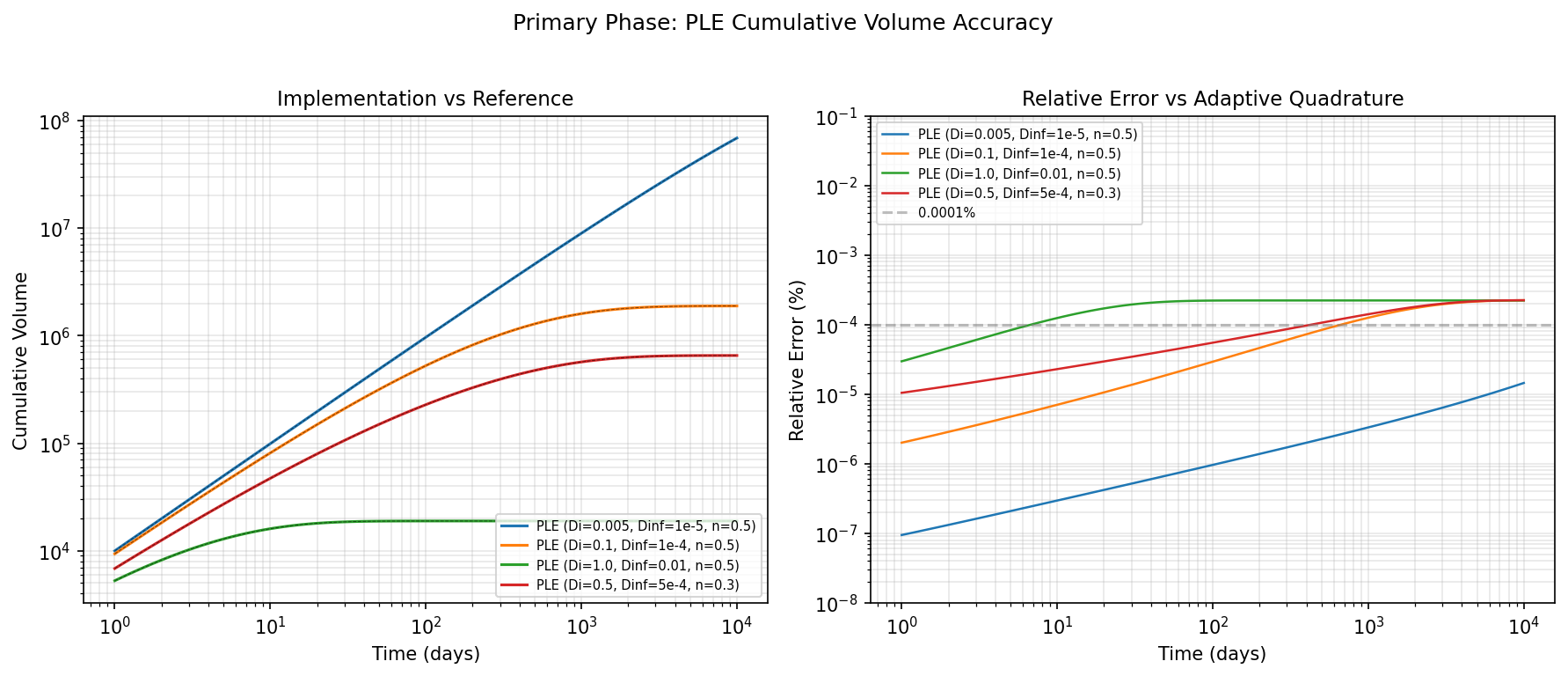
Left: cumulative volume curves for four PLE parameterizations. Implementation (solid) overlays the adaptive quadrature reference (dashed black). Right: relative error vs. time for each case.
Associated Phase Accuracy
Associated phase models (PLYield) also use numerical integration.
Their cumulative volume integrates the product of the yield function
and the primary phase rate:
The following table shows accuracy for PLYield models attached to
MH (Modified Hyperbolic) primary phases, covering rising, moderate,
steep, and declining yield profiles:
The worst-case maximum relative error for the associated phase is 0.00017%, comparable to the primary phase results. The product of yield and rate is smoother than the PLE rate alone (the MH primary has an analytical rate function), which helps the trapezoidal rule.
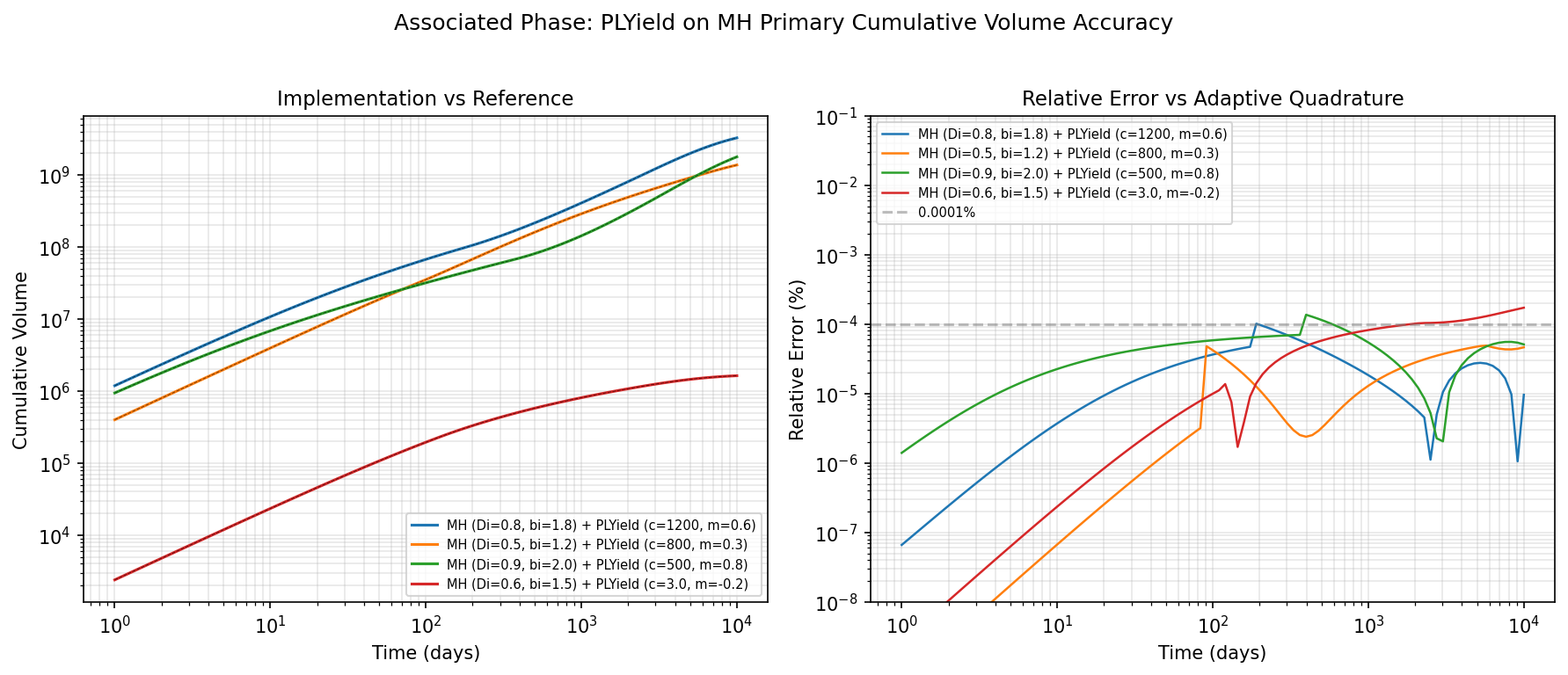
Left: cumulative secondary-phase volume for four MH + PLYield configurations. Right: relative error vs. time for each case.
Performance
The log-spaced grid approach eliminates the Python-level loop that the previous per-interval Gaussian quadrature required. All function evaluations happen in a single vectorized NumPy call, and the trapezoidal integration is performed by SciPy in compiled code.
Measured on a 101-point time array:
Method |
Time (ms) |
Max Rel Err (%) |
|---|---|---|
Per-interval fixed_quad |
~1.1 |
1.5e-04 |
Log-spaced trapezoid 10k |
~0.3 |
2.2e-04 |
The ~3x speedup comes from replacing ~100 Python-level fixed_quad
calls (each with its own function dispatch overhead) with a single
vectorized evaluation over 10,000 grid points.
Validation Script
The accuracy results above can be reproduced by running:
python docs/integration_validation.py
This script evaluates both primary phase (PLE) and associated phase (PLYield on MH) models, computes reference cumulative volumes using adaptive quadrature, and generates the accuracy figures.